Code for this analysis can be found by clicking here.

Introduction

Sampling the posterior for a likelihood conditional on discrete cluster assignment is a notoriously difficult problem for probabilistic models. Such discrete samples create a gradient discontinuity that prevents the use of gradient-based Hamiltonian Monte Carlo (HMC) samplers. This is unfortunate given the far superior efficiency of gradient-based samplers for MCMC.

Figure 1: Simulated 3-component 2-dimensional Gaussian Mixture Model.

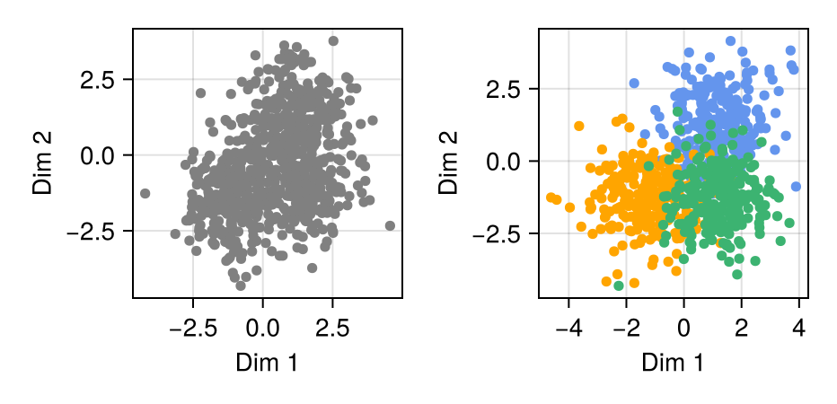
Consider the distribution shown above, which represents samples from a 3-component, 2-dimensional Gaussian Mixture Model (GMM). Turing.jl, a Julia package for Bayesian inference, is notable for its superlative ability to easily sample the full posterior of cluster assignment for each observation. However, the sampling time for even small datasets is enormously restrictive.

It is for this reason that most GMMs are implemented as marginalized models, as shown below. In a marginalized model, the cluster assignments for each point are summed out of the joint distribution. This simplifies things greatly and results in much faster fitting because the log-joint is now differentiable.

@model function gmm_standard(x, K)
    D, N = size(x)

    μ ~ filldist(MvNormal(Zeros(D), I), K)
    w ~ Dirichlet(K, 1.0)

    x ~ MixtureModel([MvNormal(μ[:, k], I) for k in 1:K], w)
end

The Smearing Problem

The weights “w” in the code above represent how strong each gaussian is in the mixture. Standard marginalized models suffer from the fact that the Dirichlet distribution and/or any Softmax-based learned weights tend to be “dense,” or non-sparse. This results in probability mass being smeared across clusters that should essentially have zero probability.

We can observe this behavior in the REPL execution below. Note how softmax assigns substantial non-zero probability to every element, whereas project_to_simplex (Sparsemax) is capable of allocating true zeros.

Function Call	Output Vector	Interpretation
softmax([1, 2, 3])	[0.090, 0.245, 0.665]	Dense: All clusters have mass.
project_to_simplex([1, 2, 3])	[0.0, 0.0, 1.0]	Sparse: Converges to a "hard" assignment (One-hot).
project_to_simplex([1, 2.9, 3])	[0.0, 0.45, 0.55]	Mixture: Sparse, but handles ambiguity.

This makes GMMs tricky to fit – because often the true number of clusters $K$ is not known ahead of time. Sparsity offers a way to fix this – by giving unlikely clusters probability 0.

Sparsemax

Wang and Carreira-Perpiñán (2013) provide an interesting method for projecting any vector of reals onto a probability simplex. This projection has the fascinating property of being able to project—differentiably—to a one-hot vector.

If inputs fall within a specific radius of the $\max x$, the vector retains mixture characteristics; otherwise, it snaps to a one-hot encoding. This property gives the method something along the lines of a “super-power,” allowing for both mixtures and discrete cluster assignments while maintaining the differentiability required for HMC.

We can implement this in a Turing model as follows:

function project_to_simplex(y::Vector{T}) where T <: Real 
    
    μ = sort(y, rev = true)

    ρ = 1
    current_sum = zero(T) 
    sum_at_ρ = zero(T)

    for j in 1:D
        current_sum += μ[j]

        if μ[j] + (1 / j) * (1 - current_sum) > 0
            ρ = j
            sum_at_ρ = current_sum
        end
    end


    λ = (1 / ρ) * (1 - sum_at_ρ) 
    
    return max.(y .+ λ, zero(T)) 
end

@model function gmm_sparsemax(x, K, temperature)
    D, N = size(x)

    μ ~ filldist(MvNormal(Zeros(D), I), K)
    
    # Learnable scaling factor for the logits
    α ~ Exponential(0.5)
    
    logits ~ filldist(Gumbel(), K)

    w = project_to_simplex(logits ./ α)

    x ~ MixtureModel([MvNormal(μ[:, k], I) for k in 1:K], w)
end

Results & Validation

This non-linear transformation can be applied to induce sparsity in the learned weight vector for the marginalized GMM. It is interesting to note the similarity to the stick-breaking process used in the marginal approximation to the “infinite” Gaussian Mixture Model. Therefore, I sought to determine if Sparsemax would produce similar results to stick-breaking and improve model fitting over a standard Dirichlet marginalized GMM.

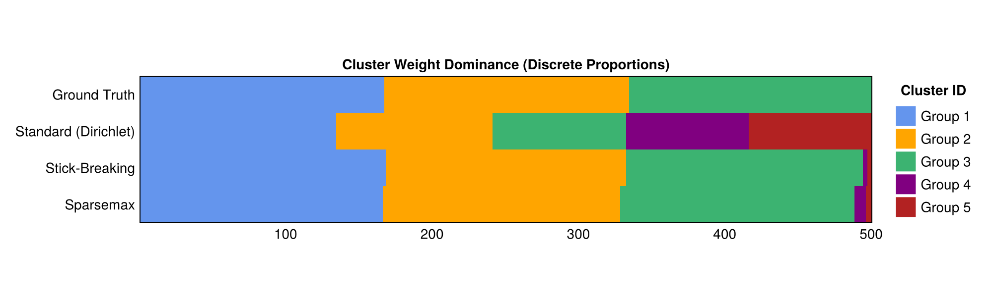
To do this, I estimated a Standard GMM, a Stick-breaking GMM, and a Sparsemax GMM with $K = 5$ to examine how robust each model was to misspecification (fitting 5 clusters to data generated from 3). Cluster assignments were visualized by taking the weights—e.g., w = sparsemax(logits / α)—and visualizing them as a proportion of a unit stick.

Posterior Weights Analysis

The figure below shows that the standard GMM fails to learn the correct weight structure, assigning significant weight to two clusters that do not actually exist.

To read the figure, consider the following. The weights $w$ must sum to 1, $\sum_{k\in K}w_k = 1$. The area for each color is proportional to the estimated cluster “representation” in the fitted model. Clearly, the standard GMM is failing to identify the correct clustering behavior in the data.

Figure 2: Heatmap comparison of learned weights $w$. Note the noise in the Standard GMM vs. the sparsity in Stick-Breaking and Sparsemax.

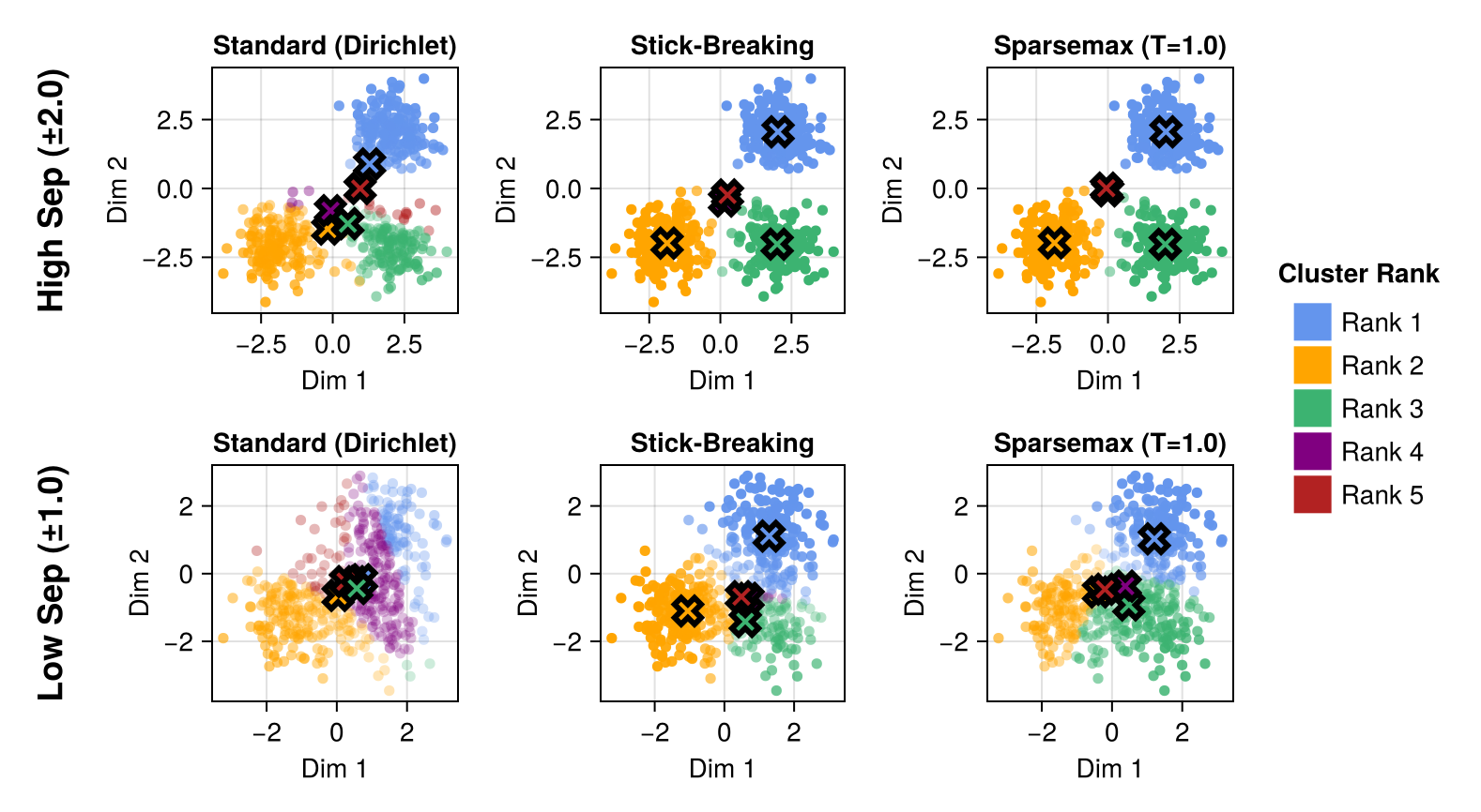
Cluster Separation

Both the stick-breaking and Sparsemax models induce significant sparsity into the model while remaining fully differentiable. Indeed, it appears that the overall results for stick-breaking and Sparsemax are nearly identical. Both have nearly identical distributions for the weights $w$, and both appear to discriminate cluster membership well, even for low-separation data.

Figure 3: Points colored by most likely cluster assignment with opacity indicating confidence of assignment.

Discussion & Conclusion

The simplex projection (Sparsemax) offers a compelling alternative to traditional Softmax or Dirichlet-based parameterizations. By allowing the model to hit “hard zeros” in the weight vector, we achieve a level of interpretability usually reserved for discrete sampling methods, without sacrificing the gradients necessary for efficient MCMC.

While the Stick-breaking process yields similar results in this experiment, Sparsemax offers distinct theoretical advantages. Stick-breaking imposes an ordering on the clusters (the “rich get richer” phenomenon), which can sometimes be undesirable depending on the prior knowledge of the data. Sparsemax, conversely, treats the logits symmetrically before projection.

For practitioners using Julia and Turing.jl, this implies that we can build models that are both sparse (interpretable) and fast (differentiable). Future work might explore how this projection behaves in higher-dimensional latent spaces, such as those found in Variational Autoencoders (VAEs), where “disentanglement” is often a primary goal.